pacman::p_load(igraph, tidygraph, ggraph,
               visNetwork, lubridate, clock,
               tidyverse, graphlayouts,
concaveman, ggforce, jsonlite, dplyr)Sailor Shift: Rise and Resonance
Getting Start
Installing and loading the required libraries
Importing data
t_data <- fromJSON("data/MC1_graph.json",
                   simplifyDataFrame = TRUE)
1. Introduction
Sailor Shift is one of the most influential figures in the development of “Oceans Folk” music. From her humble beginnings as a singer on Oceanus Island to her current status as a global superstar, she has grown to represent not only her own personal success, but has also propelled this niche genre into the world. This project uses data analysis and visualization to delve deeper into her network of collaborations, musical influences, and her importance in the overall music ecosystem. We will reveal how she has influenced others and been shaped by the zeitgeist, and further reflect on what her rise reveals about the new generation of musicians.
2. Data processing
2.1. Extracting Edges and Nodes
nodes_tbl <- as_tibble(t_data$nodes)
edges_tbl <- as_tibble(t_data$links)
2.2. Get closer to data
2.2.1. Edges

glimpse(edges_tbl)Rows: 37,857
Columns: 4
$ `Edge Type` <chr> "InterpolatesFrom", "RecordedBy", "PerformerOf", "Composer…
$ source <int> 0, 0, 1, 1, 2, 2, 3, 5, 5, 5, 5, 5, 5, 5, 5, 5, 5, 5, 5, 5…
$ target <int> 1841, 4, 0, 16180, 0, 16180, 0, 5088, 14332, 11677, 2479, …
$ key <int> 0, 0, 0, 0, 0, 0, 0, 0, 0, 0, 0, 0, 0, 0, 0, 0, 0, 0, 0, 0…length(unique(edges_tbl$`Edge Type`))[1] 12unique(edges_tbl$`Edge Type`) [1] "InterpolatesFrom" "RecordedBy" "PerformerOf"
[4] "ComposerOf" "ProducerOf" "InStyleOf"
[7] "LyricalReferenceTo" "CoverOf" "DistributedBy"
[10] "MemberOf" "LyricistOf" "DirectlySamples" The edges dataset contains 37,857 records and 4 fields to represent the various relationships between entities in the network. Each edge contains the node IDs (source and target) of the starting and ending points, as well as 12 Edge Types describing the nature of the relationship, such as “PerformerOf”, ‘ComposerOf’ or “RecordedBy”. Meanwhile, the key field is used to distinguish between multiple connections between the same node pair.
2.2.2. Nodes
glimpse(nodes_tbl)Rows: 17,412
Columns: 10
$ `Node Type` <chr> "Song", "Person", "Person", "Person", "RecordLabel", "S…
$ name <chr> "Breaking These Chains", "Carlos Duffy", "Min Qin", "Xi…
$ single <lgl> TRUE, NA, NA, NA, NA, FALSE, NA, NA, NA, NA, TRUE, NA, …
$ release_date <chr> "2017", NA, NA, NA, NA, "2026", NA, NA, NA, NA, "2020",…
$ genre <chr> "Oceanus Folk", NA, NA, NA, NA, "Lo-Fi Electronica", NA…
$ notable <lgl> TRUE, NA, NA, NA, NA, TRUE, NA, NA, NA, NA, TRUE, NA, N…
$ id <int> 0, 1, 2, 3, 4, 5, 6, 7, 8, 9, 10, 11, 12, 13, 14, 15, 1…
$ written_date <chr> NA, NA, NA, NA, NA, NA, NA, NA, NA, NA, "2020", NA, NA,…
$ stage_name <chr> NA, NA, NA, NA, NA, NA, NA, NA, NA, NA, NA, NA, NA, NA,…
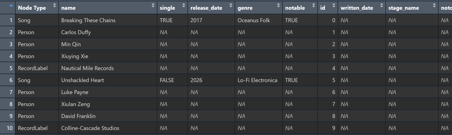
$ notoriety_date <chr> NA, NA, NA, NA, NA, NA, NA, NA, NA, NA, NA, NA, NA, NA,…The nodes dataset contains 17,412 entries, each representing an entity within the music network and categorized under the Node Type column as “Person”, “Song”, or “RecordLabel”. Each node includes relevant attributes based on its type—for example, songs have fields such as single, release_date, genre, and notable, while people may have stage_name and notoriety_date. The presence of missing values (NA) in many fields indicates that certain attributes are only applicable to specific node types.
2.2.3. Initial EDA
ggplot(data = edges_tbl,
       aes(y = `Edge Type`)) +
  geom_bar()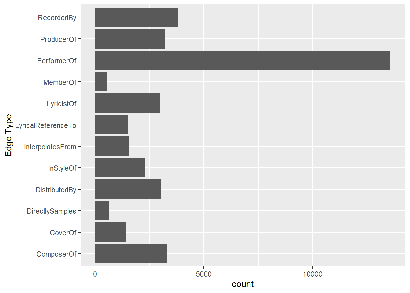
This bar chart above shows the distribution of different edge types in the music relationship network. The most common type is PerformerOf, indicating that the data heavily captures who performed which work. Other frequent types include ComposerOf, LyricistOf, and ProducerOf, highlighting the importance of creative and production roles. In contrast, relationships like MemberOf and DirectlySamples are less common, suggesting these connections are either rarer or less documented.
ggplot(data = nodes_tbl,
       aes(y = `Node Type`)) +
  geom_bar()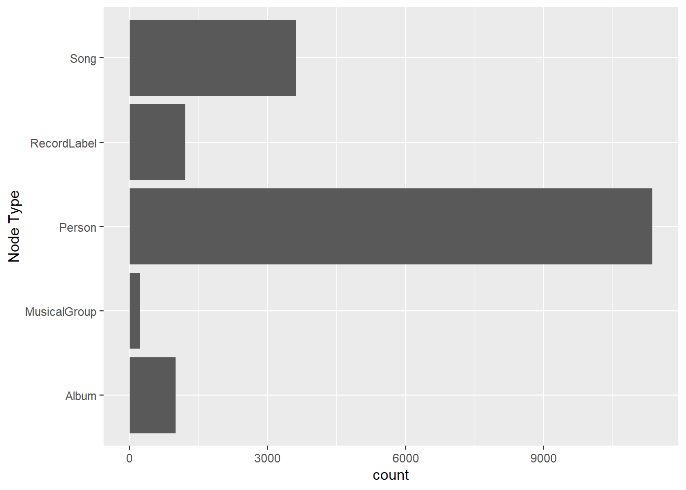
This bar chart displays the distribution of different node types in the music network dataset. The most common type is Person, with a count far exceeding other categories, indicating a strong focus on individual artists, producers, and contributors. Songs also appear in large numbers, highlighting the dataset’s emphasis on works being created or performed. Other types like Albums, RecordLabels, and MusicalGroups are present but in significantly smaller quantities.
3. Creating Knowledge Graph
3.1. Mapping from node id to row index
id_map <- tibble(id = nodes_tbl$id,
                 index = seq_len(
                   nrow(nodes_tbl)))
3.2. Map source and target IDs to row indices
edges_tbl <- edges_tbl %>%
  left_join(id_map, by = c("source" = "id")) %>%
  rename(from = index) %>%
  left_join(id_map, by = c("target" = "id")) %>%
  rename(to = index)
3.3. Filter out any unmatched (invalid) edges
edges_tbl <- edges_tbl %>%
  filter(!is.na(from), !is.na(to))
3.4. Creating tidygraph
graph <- tbl_graph(nodes = nodes_tbl,
                   edges = edges_tbl,
directed = t_data$directed)class(graph)[1] "tbl_graph" "igraph" 4. Visualising the knowledge graph
set.seed(1234)4.1. Visualising the whole graph
ggraph(graph, layout = "fr") +
  geom_edge_link(alpha = 0.3,
                 colour = "gray") +
  geom_node_point(aes(color = `Node Type`),
                  size = 4) +
  geom_node_text(aes(label = name),
                 repel = TRUE,
                 size = 2.5) +
  theme_void()
4.2. Visualising the sub-graph
4.2.1. Filtering edges to only “MemberOf”
graph_memberof <- graph %>%
  activate(edges) %>%
  filter(`Edge Type` == "MemberOf")
4.2.2. Extracting only connected nodes (i.e., used in these edges)
used_node_indices <- graph_memberof %>%
  activate(edges) %>%
  as_tibble() %>%
  select(from, to) %>%
  unlist() %>%
  unique()
4.2.3. Keeping only those nodes
graph_memberof <- graph_memberof %>%
  activate(nodes) %>%
  mutate(row_id = row_number()) %>%
  filter(row_id %in% used_node_indices) %>%
  select(-row_id)  # optional cleanup
4.2.4. Plotting the sub-graph
ggraph(graph_memberof,
       layout = "fr") +
  geom_edge_link(alpha = 0.5,
                 colour = "gray") +
  geom_node_point(aes(color = `Node Type`),
                  size = 1) +
  geom_node_text(aes(label = name),
                 repel = TRUE,
                 size = 2.5) +
  theme_void()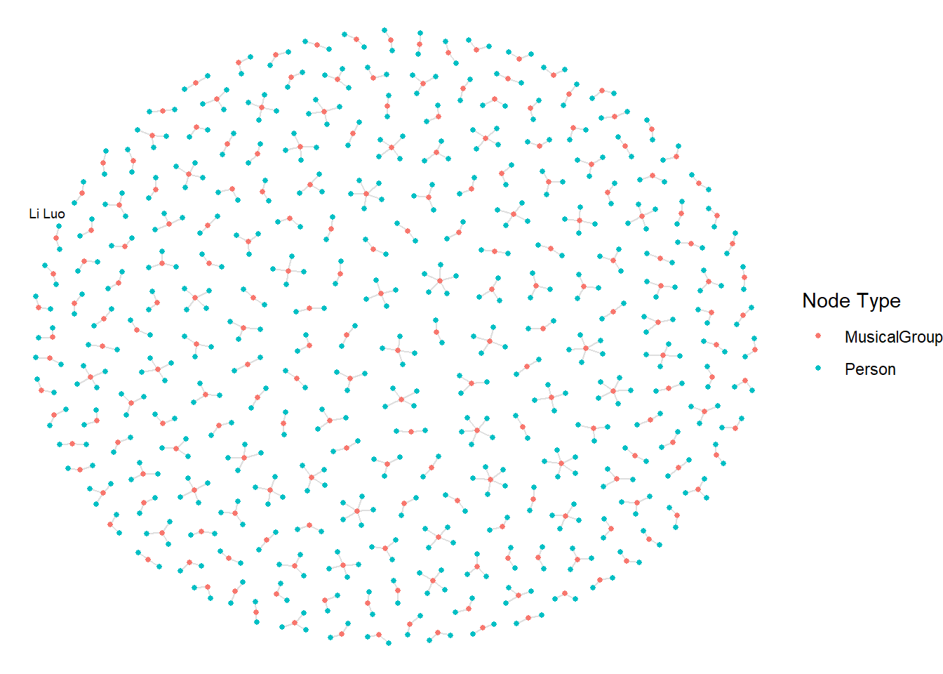
5. Sailor Shift’s Career Connections
5.1. The contributors who shaped the modern Sailor Shift
A singer’s journey to fame is never a solitary one. Sailor has been accompanied by many — fellow singers, producers, instrumentalists, composers, and others who helped shape her path.
# Sailor Shift's Index
sailor_idx <- which(nodes_tbl$name == "Sailor Shift")
# Sailor Shift's works'Index
perf_edges <- graph %>%
activate(edges) %>%
as_tibble() %>%
filter(`Edge Type` == "PerformerOf", from == sailor_idx)
sailor_works_idx <- perf_edges %>% pull(to) %>% unique()
focus_idx1 <- unique(c(sailor_idx, sailor_works_idx))# Keep Edges that 'influence' Sailor Shift's works
influence_types1 <- c("ComposerOf", "ProducerOf", "LyricistOf", "CoverOf")
graph_influence1 <- graph %>%
activate(edges) %>%
filter(
`Edge Type` %in% influence_types1,
to %in% focus_idx1
)# Extract Nodes
used_node_indices1 <- graph_influence1 %>%
activate(edges) %>%
as_tibble() %>%
select(from, to) %>%
unlist() %>%
unique()# Keep Nodes
graph_influence1 <- graph_influence1 %>%
activate(nodes) %>%
mutate(.row = row_number()) %>%
filter(.row %in% used_node_indices1) %>%
select(-.row)# Plot
ggraph(graph_influence1, layout = "fr") +
geom_edge_link(aes(color = `Edge Type`),
arrow = arrow(length = unit(4, "pt"), type = "closed"),
end_cap = circle(3, "pt"),
start_cap = circle(3, "pt"),
width = 0.5,
alpha = 0.6,
show.legend = TRUE) +
geom_node_point(aes(color = `Node Type`),
size = 2) +
geom_node_text(aes(label = name),
size = 2.5,
repel = TRUE,
max.overlaps = Inf) +
scale_edge_colour_brewer(palette = "Set2",
name = "Edge Type") +
scale_color_manual(values = c(
"Person" = "#377EB8",
"Album" = "#E41A1C",
"RecordLabel" = "#4DAF4A"
), name = "Node Type") +
theme_void() +
theme(
legend.position = "right",
legend.title = element_text(size = 10),
legend.text = element_text(size = 8),
plot.margin = margin(5, 5, 5, 5)
)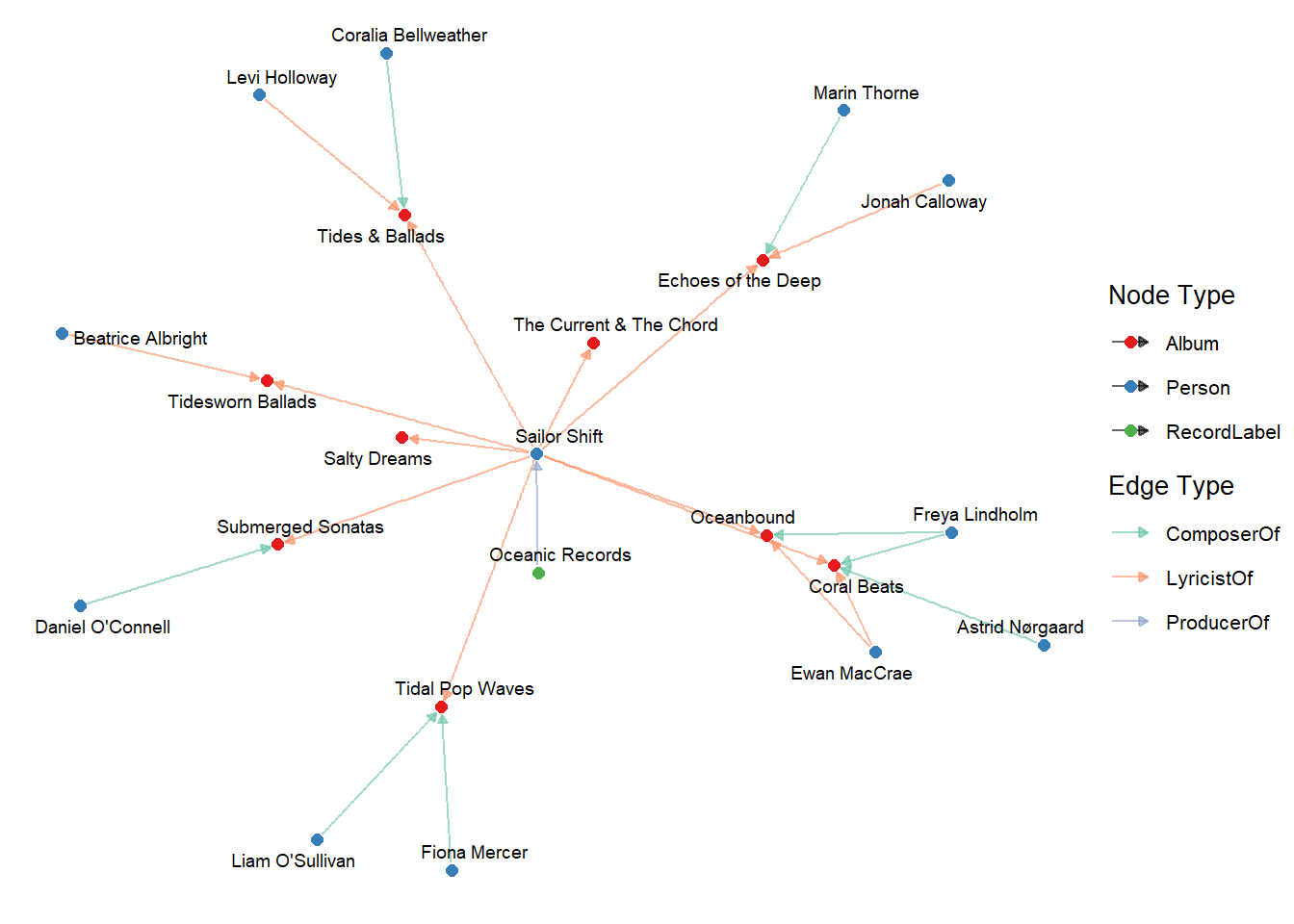
This network diagram places Sailor Shift at its center and reveals the diverse teams behind each album. By mapping the ComposerOf, ProducerOf and LyricistOf relationships, it clearly shows which composers, producers, and record labels have shaped her work. From the visualization, it’s clear that Ewan MacRae has had the greatest influence on her discography: he not only composed Oceanbound alone but also teamed up with Freya Lindholm and Astrid Nørgaard to co-create Coral Beats, leaving a significant mark on two albums—far more than any other contributor.
5.2. Who did Sailor Shift influenced
Throughout Sailor’s career, not only has Sailor received influences from others, but her work has begun to inspire others, extending her creative reach beyond her immediate circle.
# Sailor's works
layer1_targets <- perf_edges %>%
  pull(to)
# Works influenced by Silor's works
influence_types2 <- c("DirectlySamples", "InStyleOf",
"LyricalReferenceTo", "InterpolatesFrom")
layer2_targets <- graph %>%
activate(edges) %>%
as_tibble() %>%
filter(`Edge Type` %in% influence_types2,
from %in% layer1_targets) %>%
pull(to)# Creators of those influenced works
creator_types <- c("ComposerOf", "ProducerOf", "LyricistOf")
graph_sub2 <- graph %>%
activate(edges) %>%
filter(
(`Edge Type` == "PerformerOf" & from == sailor_idx) |
(`Edge Type` %in% influence_types2 & from %in% layer1_targets) |
(`Edge Type` %in% creator_types & to %in% layer2_targets)
)
used_nodes2 <- graph_sub2 %>%
activate(edges) %>%
as_tibble() %>%
select(from, to) %>%
unlist() %>%
unique()
graph_sub2 <- graph_sub2 %>%
activate(nodes) %>%
mutate(.row = row_number()) %>%
filter(.row %in% used_nodes2) %>%
select(-.row)
ggraph(graph_sub2, layout = "fr") +
geom_edge_link(aes(color = `Edge Type`),
arrow = arrow(length = unit(3, "pt"), type = "closed"),
end_cap = circle(2.5, "pt"),
start_cap = circle(2.5, "pt"),
width = 0.6,
alpha = 0.7) +
geom_node_point(aes(color = `Node Type`), size = 3) +
geom_node_text(aes(label = name), repel = TRUE, size = 2.5, max.overlaps = Inf) +
scale_edge_colour_manual(values = c(
PerformerOf = "#8DD3C7",
DirectlySamples = "#FB8072",
InStyleOf = "#80B1D3",
LyricalReferenceTo = "#FDB462",
InterpolatesFrom = "#B3DE69",
ComposerOf = "#FCCDE5",
ProducerOf = "#BEBADA",
LyricistOf = "#FFED6F"
), name = "Relation") +
scale_color_manual(values = c(
Person = "#377EB8",
Album = "#E41A1C",
Song = "#4DAF4A",
RecordLabel = "#984EA3",
MusicalGroup = "#FF7F00"
), name = "Node Type") +
theme_void() +
theme(
legend.position = "right",
legend.title = element_text(size = 10),
legend.text = element_text(size = 8)
)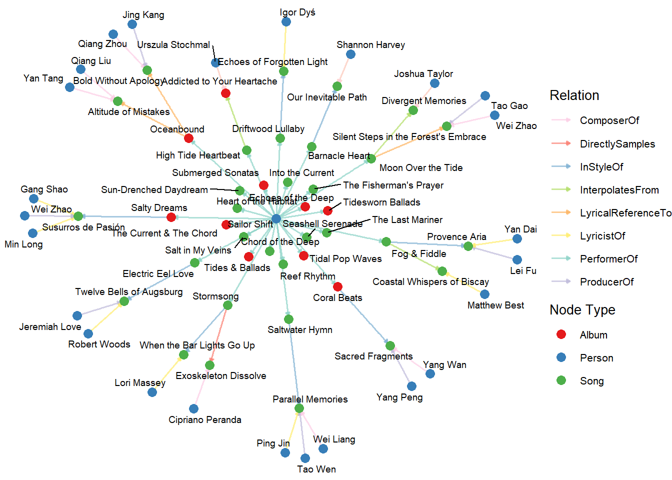
This visualization adopts a four-layer peeling approach: at the very center sits Sailor Shift (blue), surrounded by her own recordings and lyric-penned tracks (red and green). The third ring maps the songs that directly sample, stylistically echo, lyrically reference, or interpolate her work (green), and the outermost layer identifies the composers, producers, and lyricists (blue) behind those derivative pieces. By counting connection frequencies, Wei Zhao stands out as the most heavily influenced creator—appearing under two separate derivative tracks—making them the single individual most shaped by Sailor Shift’s musical legacy.
5.3. Sailor Shift‘s influence to the Oceanus Folk community
# Sailor's Index
sailor_idx <- which(nodes_tbl$name == "Sailor Shift")
# Sailor's works
creative_edge_types <- c("PerformerOf")
perf_edges <- graph %>%
activate(edges) %>%
as_tibble() %>%
filter(`Edge Type` %in% creative_edge_types, from == sailor_idx)
sailor_works_idx <- perf_edges %>% pull(to) %>% unique()nodes_tbl[sailor_works_idx, ]# A tibble: 26 × 10
`Node Type` name single release_date genre notable id written_date
<chr> <chr> <lgl> <chr> <chr> <lgl> <int> <chr>
1 Album Tidal Pop W… NA 2028 Ocea… TRUE 17272 2027
2 Album Salty Dreams NA 2030 Ocea… TRUE 17273 2029
3 Album The Current… NA 2032 Ocea… TRUE 17274 2031
4 Album Coral Beats NA 2034 Ocea… TRUE 17275 2033
5 Album Tides & Bal… NA 2036 Ocea… TRUE 17276 2035
6 Album Oceanbound NA 2038 Ocea… TRUE 17277 2037
7 Album Echoes of t… NA 2040 Ocea… TRUE 17278 2039
8 Song High Tide H… TRUE 2028 Ocea… FALSE 17279 <NA>
9 Song Electric Ee… FALSE 2028 Ocea… TRUE 17280 <NA>
10 Song Sun-Drenche… FALSE 2028 Ocea… FALSE 17281 <NA>
# ℹ 16 more rows
# ℹ 2 more variables: stage_name <chr>, notoriety_date <chr># Oceanus Folk Community works
oceanus_works_idx <- nodes_tbl %>%
mutate(idx = row_number()) %>%
filter(genre == "Oceanus Folk") %>%
pull(idx)# Combine all nodes
focus_idx <- unique(c(sailor_works_idx, oceanus_works_idx))nodes_tbl[focus_idx, ]# A tibble: 305 × 10
`Node Type` name single release_date genre notable id written_date
<chr> <chr> <lgl> <chr> <chr> <lgl> <int> <chr>
1 Album Tidal Pop W… NA 2028 Ocea… TRUE 17272 2027
2 Album Salty Dreams NA 2030 Ocea… TRUE 17273 2029
3 Album The Current… NA 2032 Ocea… TRUE 17274 2031
4 Album Coral Beats NA 2034 Ocea… TRUE 17275 2033
5 Album Tides & Bal… NA 2036 Ocea… TRUE 17276 2035
6 Album Oceanbound NA 2038 Ocea… TRUE 17277 2037
7 Album Echoes of t… NA 2040 Ocea… TRUE 17278 2039
8 Song High Tide H… TRUE 2028 Ocea… FALSE 17279 <NA>
9 Song Electric Ee… FALSE 2028 Ocea… TRUE 17280 <NA>
10 Song Sun-Drenche… FALSE 2028 Ocea… FALSE 17281 <NA>
# ℹ 295 more rows
# ℹ 2 more variables: stage_name <chr>, notoriety_date <chr># Influence Types
influence_types3 <- c(
"DirectlySamples",
"InStyleOf",
"LyricalReferenceTo",
"InterpolatesFrom",
"CoverOf"
)# Filter Edges
graph_3 <- graph %>%
activate(edges) %>%
filter(`Edge Type` %in% influence_types3 )# Extracting Nodes
used_node_indices3 <- graph_3 %>%
activate(edges) %>%
as_tibble() %>%
select(from, to) %>%
unlist() %>%
unique()# Keep Nodes
graph_3 <- graph_3 %>%
activate(nodes) %>%
mutate(row_id = row_number()) %>%
filter(row_id %in% focus_idx) %>%
select(-row_id) # optional cleanup# Add label
graph_3 <- graph_3 %>%
activate(nodes) %>%
mutate(is_sailor_work = ifelse(name %in% nodes_tbl$name[sailor_works_idx],
"Sailor's Work", "Other"))# Ploting
ggraph(graph_3, layout = "fr") +
geom_edge_link(alpha = 0.5, colour = "gray") +
geom_node_point(aes(color = is_sailor_work), size = 1.5) +
theme_void()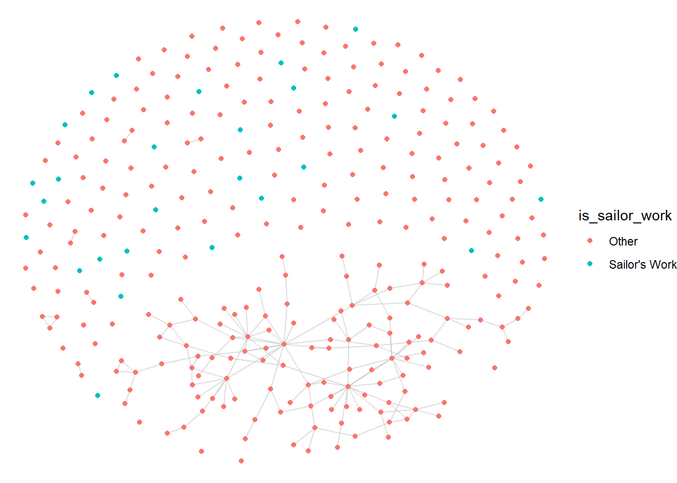
Sailor Shift has influenced collaborators in the Oceanus Folk community primarily through indirect inspiration. Her works, though few in number, are embedded across different parts of the network, suggesting they have been referenced or sampled by multiple creators. While she doesn’t appear to collaborate repeatedly with specific individuals, her influence spans across stylistic clusters, indicating a broad and decentralized artistic impact