pacman::p_load(igraph, tidygraph, ggraph,
               visNetwork, lubridate, clock,
               tidyverse, graphlayouts,
concaveman, ggforce)Hands-on_Ex05
Getting Started
Installing and launching R packages
Importing network data
GAStech_nodes <- read_csv("data/GAStech_email_node.csv")
GAStech_edges <- read_csv("data/GAStech_email_edge-v2.csv")
Reviewing the imported data
glimpse(GAStech_edges)Rows: 9,063
Columns: 8
$ source <dbl> 43, 43, 44, 44, 44, 44, 44, 44, 44, 44, 44, 44, 26, 26, 26…
$ target <dbl> 41, 40, 51, 52, 53, 45, 44, 46, 48, 49, 47, 54, 27, 28, 29…
$ SentDate <chr> "6/1/2014", "6/1/2014", "6/1/2014", "6/1/2014", "6/1/2014"…
$ SentTime <time> 08:39:00, 08:39:00, 08:58:00, 08:58:00, 08:58:00, 08:58:0…
$ Subject <chr> "GT-SeismicProcessorPro Bug Report", "GT-SeismicProcessorP…
$ MainSubject <chr> "Work related", "Work related", "Work related", "Work rela…
$ sourceLabel <chr> "Sven.Flecha", "Sven.Flecha", "Kanon.Herrero", "Kanon.Herr…
$ targetLabel <chr> "Isak.Baza", "Lucas.Alcazar", "Felix.Resumir", "Hideki.Coc…Wrangling time
GAStech_edges <- GAStech_edges %>%
  mutate(SendDate = dmy(SentDate)) %>%
  mutate(Weekday = wday(SentDate,
                        label = TRUE,
                        abbr = FALSE))
Wrangling attributes
GAStech_edges_aggregated <- GAStech_edges %>%
  filter(MainSubject == "Work related") %>%
  group_by(source, target, Weekday) %>%
    summarise(Weight = n()) %>%
  filter(source!=target) %>%
  filter(Weight > 1) %>%
  ungroup()
Creating network objects using tidygraph
Using tbl_graph() to build tidygraph data model
GAStech_graph <- tbl_graph(nodes = GAStech_nodes,
                           edges = GAStech_edges_aggregated,
                           directed = TRUE)
Reviewing the output tidygraph’s graph object
GAStech_graph# A tbl_graph: 54 nodes and 1372 edges
#
# A directed multigraph with 1 component
#
# Node Data: 54 × 4 (active)
id label Department Title
<dbl> <chr> <chr> <chr>
1 1 Mat.Bramar Administration Assistant to CEO
2 2 Anda.Ribera Administration Assistant to CFO
3 3 Rachel.Pantanal Administration Assistant to CIO
4 4 Linda.Lagos Administration Assistant to COO
5 5 Ruscella.Mies.Haber Administration Assistant to Engineering Group Mana…
6 6 Carla.Forluniau Administration Assistant to IT Group Manager
7 7 Cornelia.Lais Administration Assistant to Security Group Manager
8 44 Kanon.Herrero Security Badging Office
9 45 Varja.Lagos Security Badging Office
10 46 Stenig.Fusil Security Building Control
# ℹ 44 more rows
#
# Edge Data: 1,372 × 4
from to Weekday Weight
<int> <int> <ord> <int>
1 1 2 Sunday 5
2 1 2 Monday 2
3 1 2 Tuesday 3
# ℹ 1,369 more rowsChanging the active object
GAStech_graph %>%
  activate(edges) %>%
  arrange(desc(Weight))
# A tbl_graph: 54 nodes and 1372 edges
#
# A directed multigraph with 1 component
#
# Edge Data: 1,372 × 4 (active)
from to Weekday Weight
<int> <int> <ord> <int>
1 40 41 Saturday 13
2 41 43 Monday 11
3 35 31 Tuesday 10
4 40 41 Monday 10
5 40 43 Monday 10
6 36 32 Sunday 9
7 40 43 Saturday 9
8 41 40 Monday 9
9 19 15 Wednesday 8
10 35 38 Tuesday 8
# ℹ 1,362 more rows
#
# Node Data: 54 × 4
id label Department Title
<dbl> <chr> <chr> <chr>
1 1 Mat.Bramar Administration Assistant to CEO
2 2 Anda.Ribera Administration Assistant to CFO
3 3 Rachel.Pantanal Administration Assistant to CIO
# ℹ 51 more rowsPlotting Static Network Graphs with ggraph package
Plotting a basic network graph
ggraph(GAStech_graph) +
  geom_edge_link() +
  geom_node_point()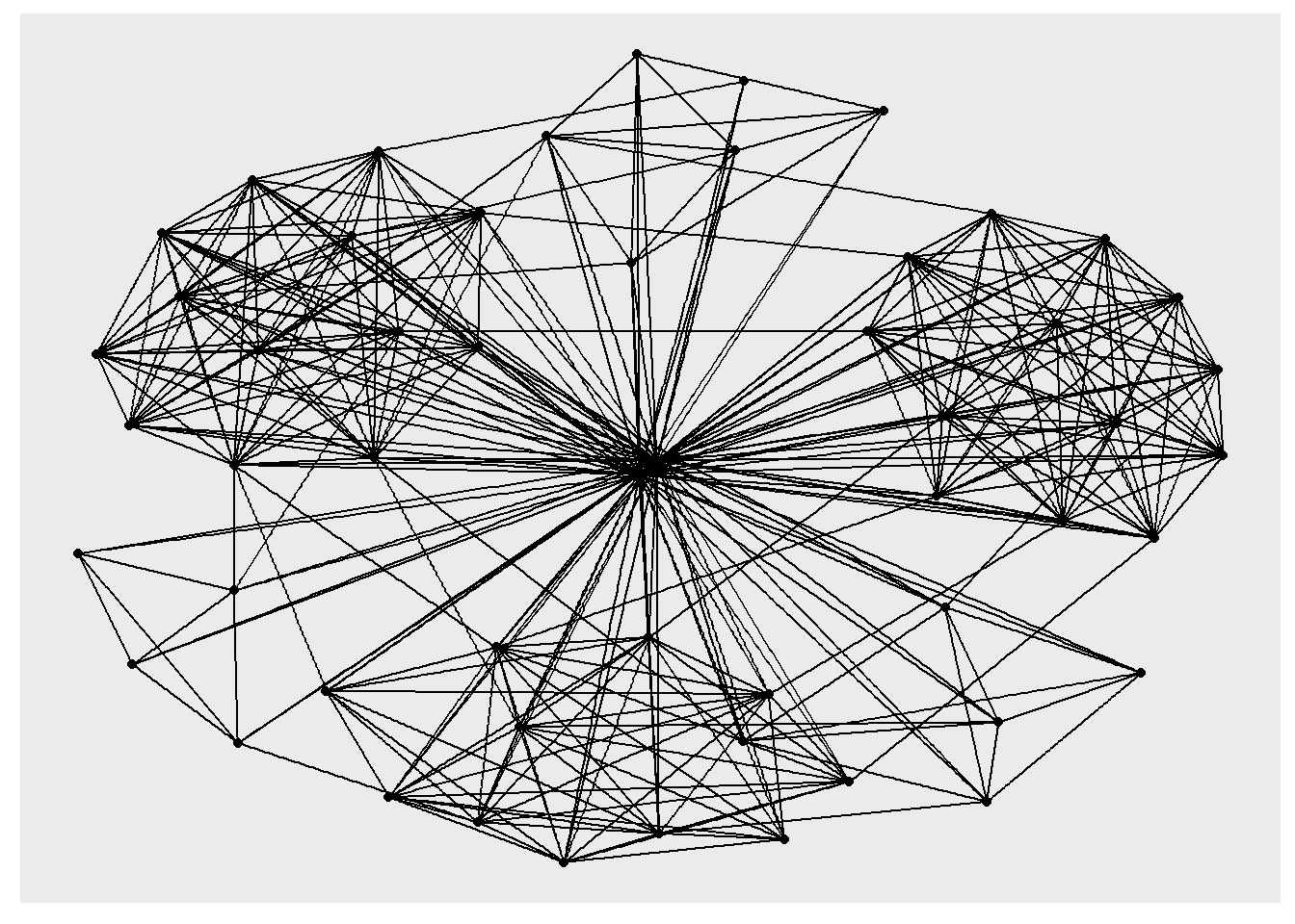
Changing the default network graph theme
g <- ggraph(GAStech_graph) +
  geom_edge_link(aes()) +
  geom_node_point(aes())

g + theme_graph()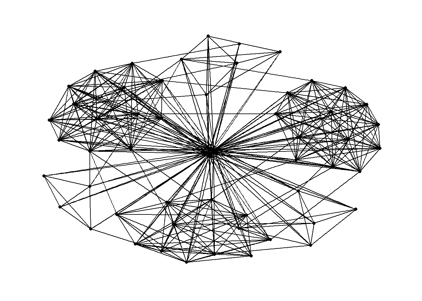
Changing the coloring of the plot
g <- ggraph(GAStech_graph) +
  geom_edge_link(aes(colour = 'grey50')) +
  geom_node_point(aes(colour = 'grey40'))

g + theme_graph(background = 'grey10',
                text_colour = 'white')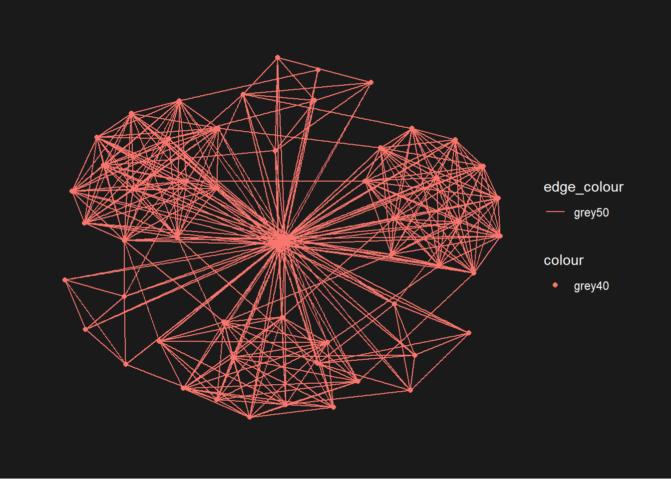
Fruchterman and Reingold layout
g <- ggraph(GAStech_graph,
            layout = "fr") +
  geom_edge_link(aes()) +
  geom_node_point(aes())

g + theme_graph()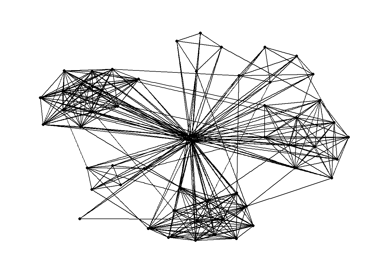
Star layout
g <- ggraph(GAStech_graph,
            layout = "star") +
  geom_edge_link(aes()) +
  geom_node_point(aes())

g + theme_graph()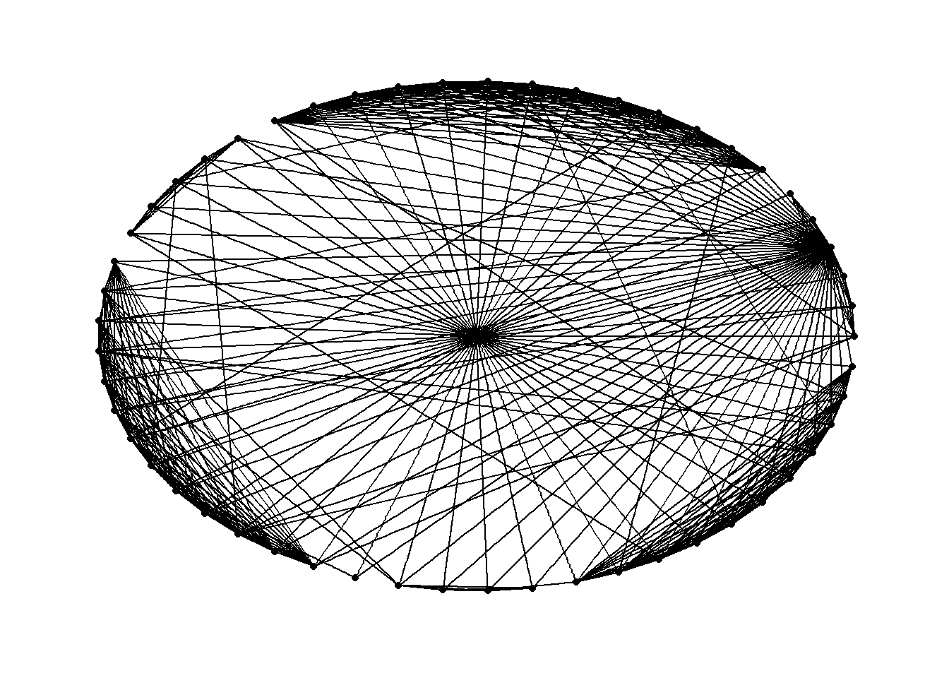
Nicely layout
g <- ggraph(GAStech_graph,
            layout = "nicely") +
  geom_edge_link(aes()) +
  geom_node_point(aes())

g + theme_graph()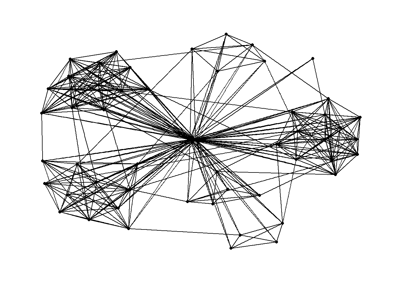
Random layout
g <- ggraph(GAStech_graph,
            layout = "randomly") +
  geom_edge_link(aes()) +
  geom_node_point(aes())

g + theme_graph()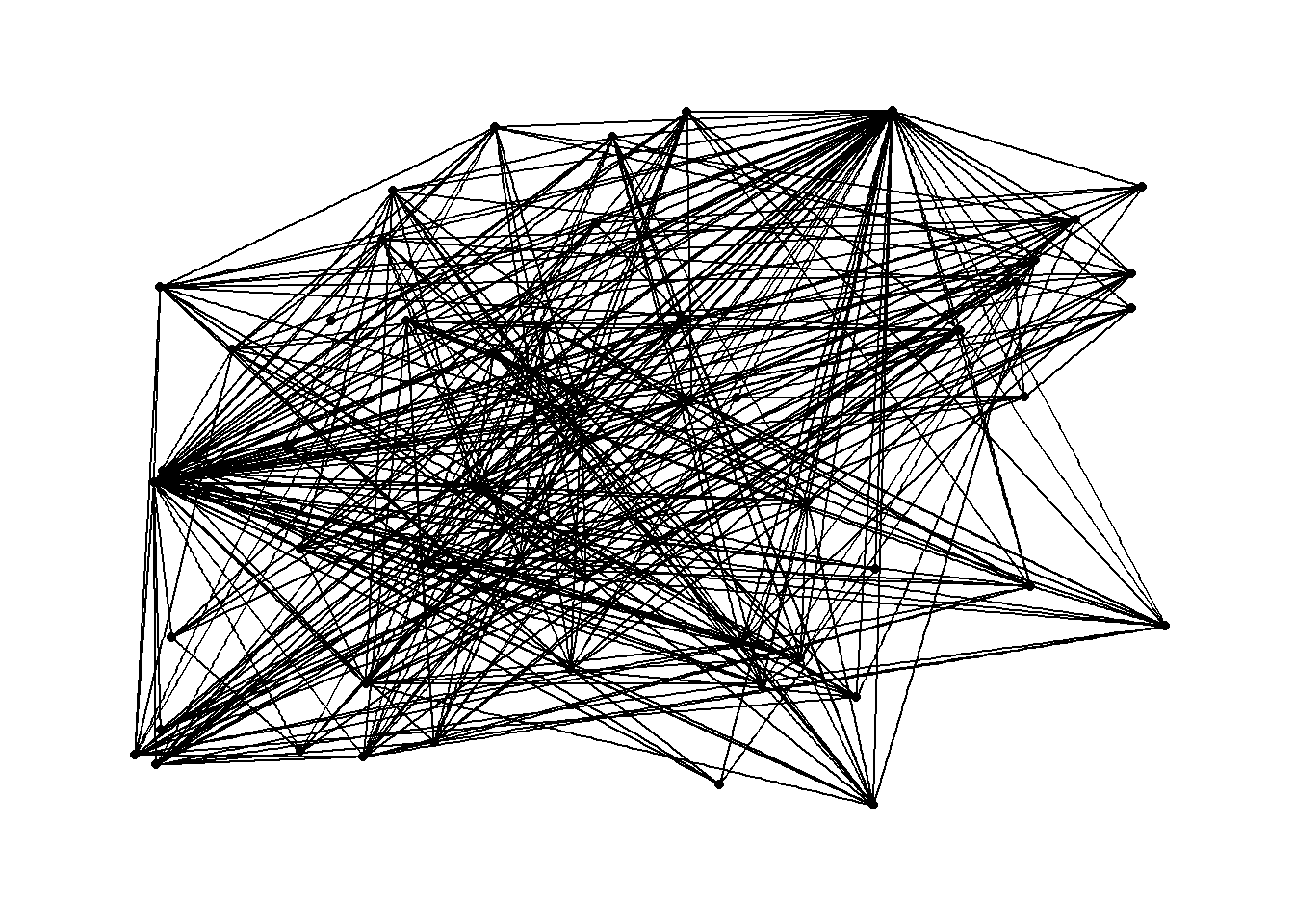
Modifying network nodes
g <- ggraph(GAStech_graph,
            layout = "nicely") +
  geom_edge_link(aes()) +
  geom_node_point(aes(colour = Department,
                      size = 3))

g + theme_graph()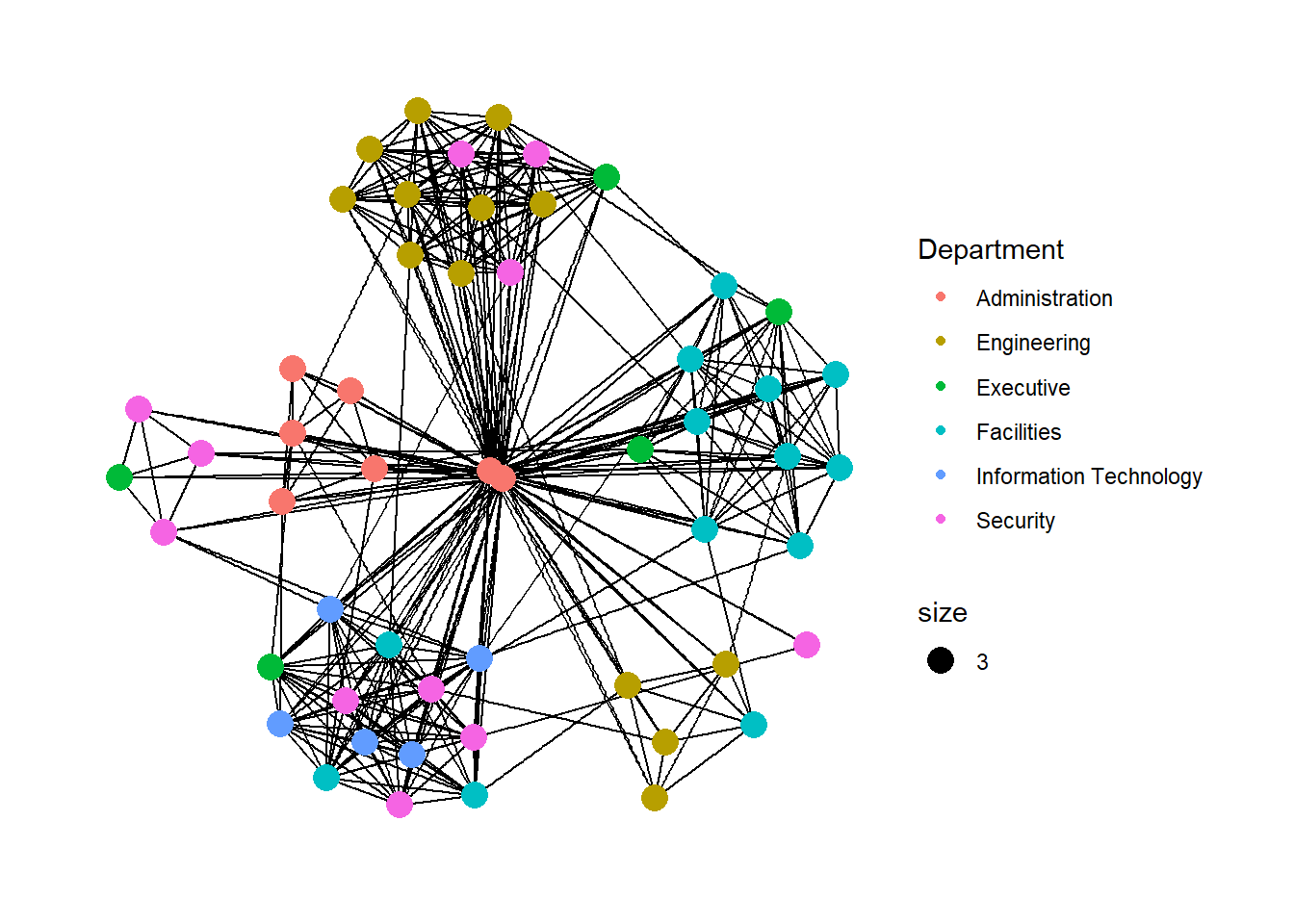
Modifying edges
g <- ggraph(GAStech_graph,
            layout = "nicely") +
  geom_edge_link(aes(width=Weight),
                 alpha=0.2) +
  scale_edge_width(range = c(0.1, 5)) +
  geom_node_point(aes(colour = Department),
                  size = 3)

g + theme_graph()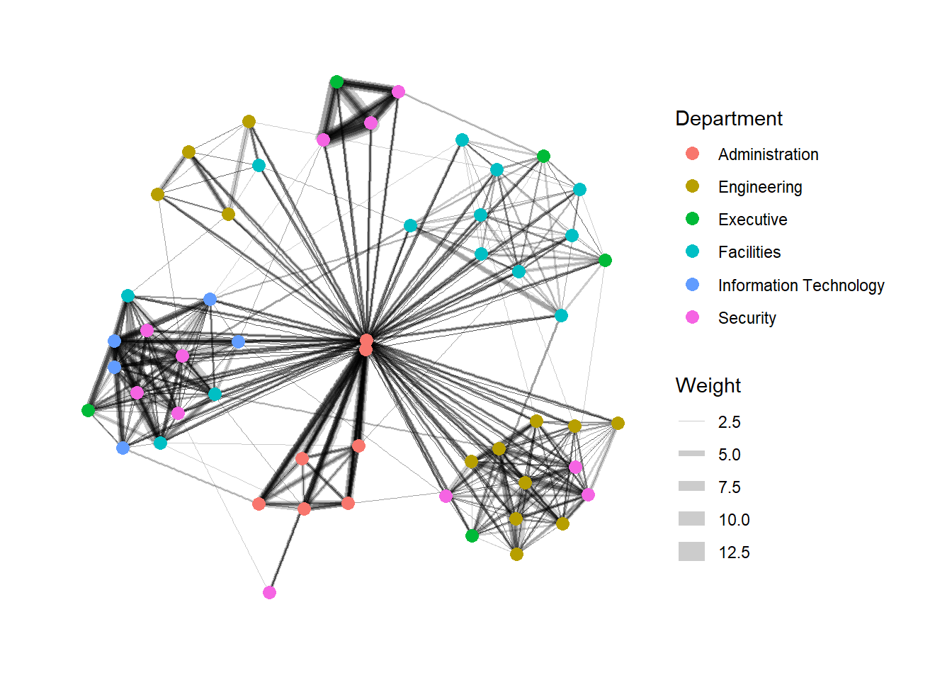
Creating facet graphs
Working with facet_edges()
set_graph_style()

g <- ggraph(GAStech_graph,
            layout = "nicely") +
  geom_edge_link(aes(width=Weight),
                 alpha=0.2) +
  scale_edge_width(range = c(0.1, 5)) +
  geom_node_point(aes(colour = Department),
                  size = 2)

g + facet_edges(~Weekday)
Working with facet_edges() and theme()
set_graph_style()

g <- ggraph(GAStech_graph,
            layout = "nicely") +
  geom_edge_link(aes(width=Weight),
                 alpha=0.2) +
  scale_edge_width(range = c(0.1, 5)) +
  geom_node_point(aes(colour = Department),
                  size = 2) +
  theme(legend.position = 'bottom')

g + facet_edges(~Weekday)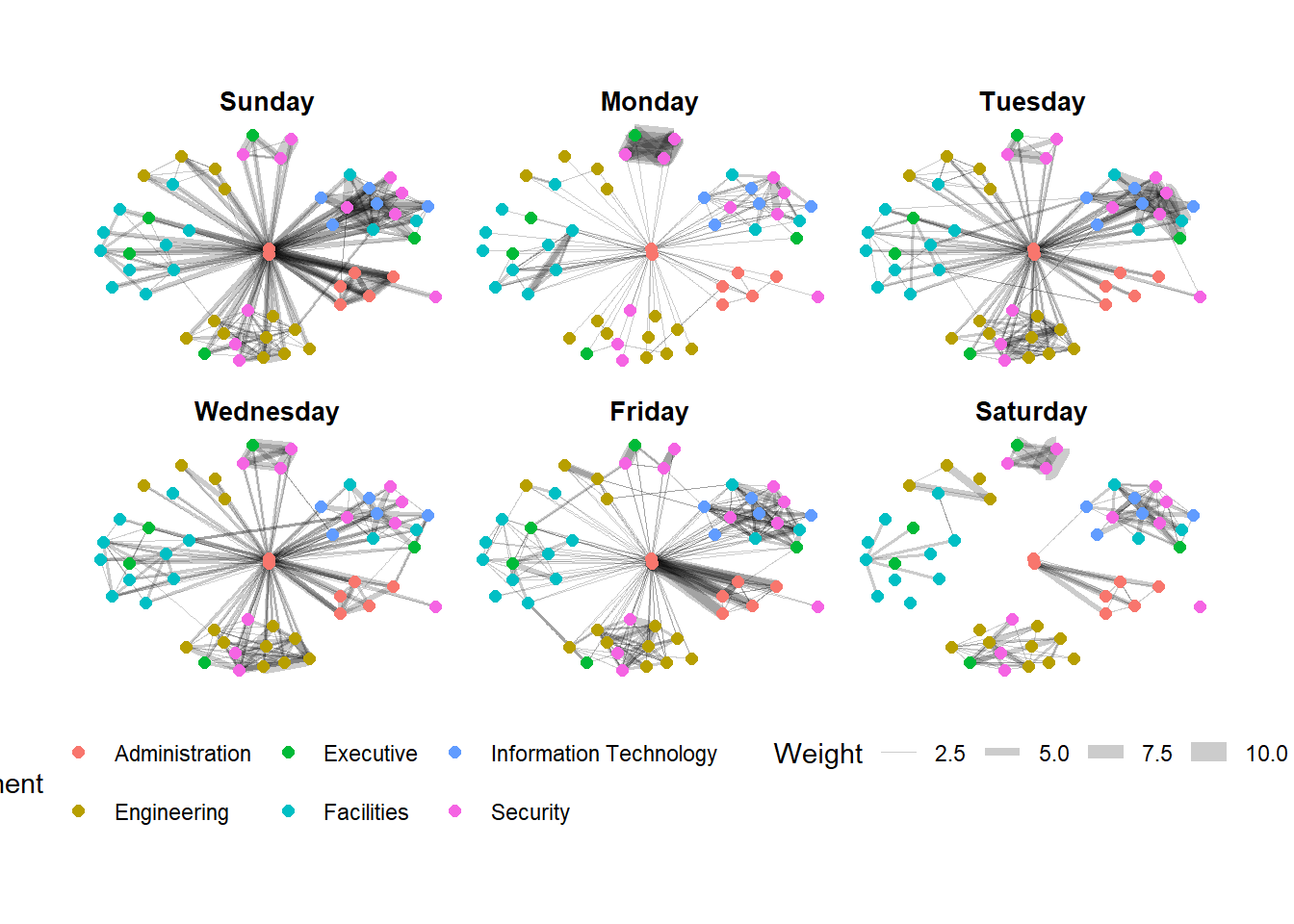
A framed facet graph
set_graph_style()

g <- ggraph(GAStech_graph,
            layout = "nicely") +
  geom_edge_link(aes(width=Weight),
                 alpha=0.2) +
  scale_edge_width(range = c(0.1, 5)) +
  geom_node_point(aes(colour = Department),
                  size = 2)

g + facet_edges(~Weekday) +
  th_foreground(foreground = "grey80",
                border = TRUE) +
  theme(legend.position = 'bottom')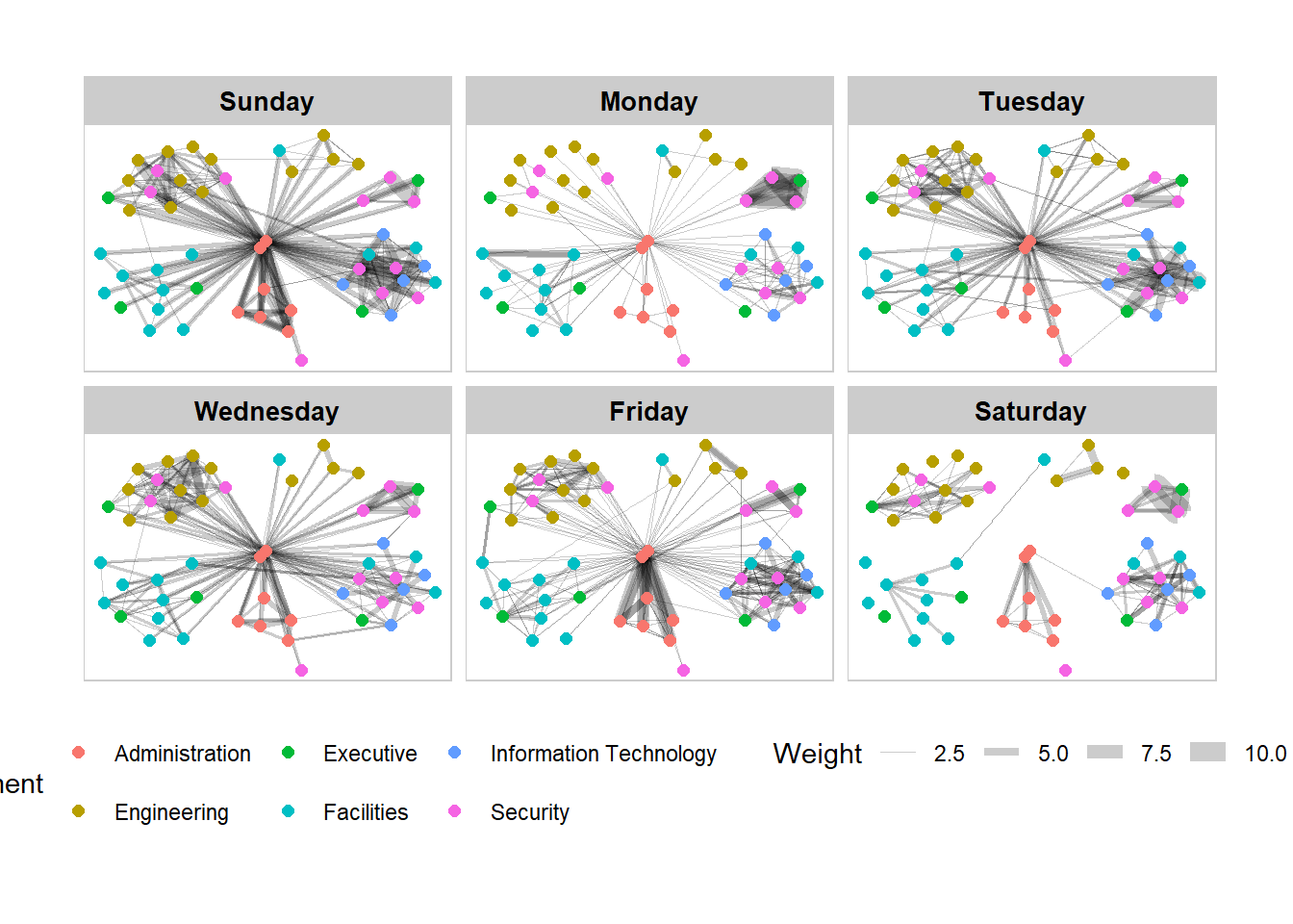
Working with facet_nodes()
set_graph_style()

g <- ggraph(GAStech_graph,
            layout = "nicely") +
  geom_edge_link(aes(width=Weight),
                 alpha=0.2) +
  scale_edge_width(range = c(0.1, 5)) +
  geom_node_point(aes(colour = Department),
                  size = 2)

g + facet_nodes(~Department)+
  th_foreground(foreground = "grey80",
                border = TRUE) +
  theme(legend.position = 'bottom')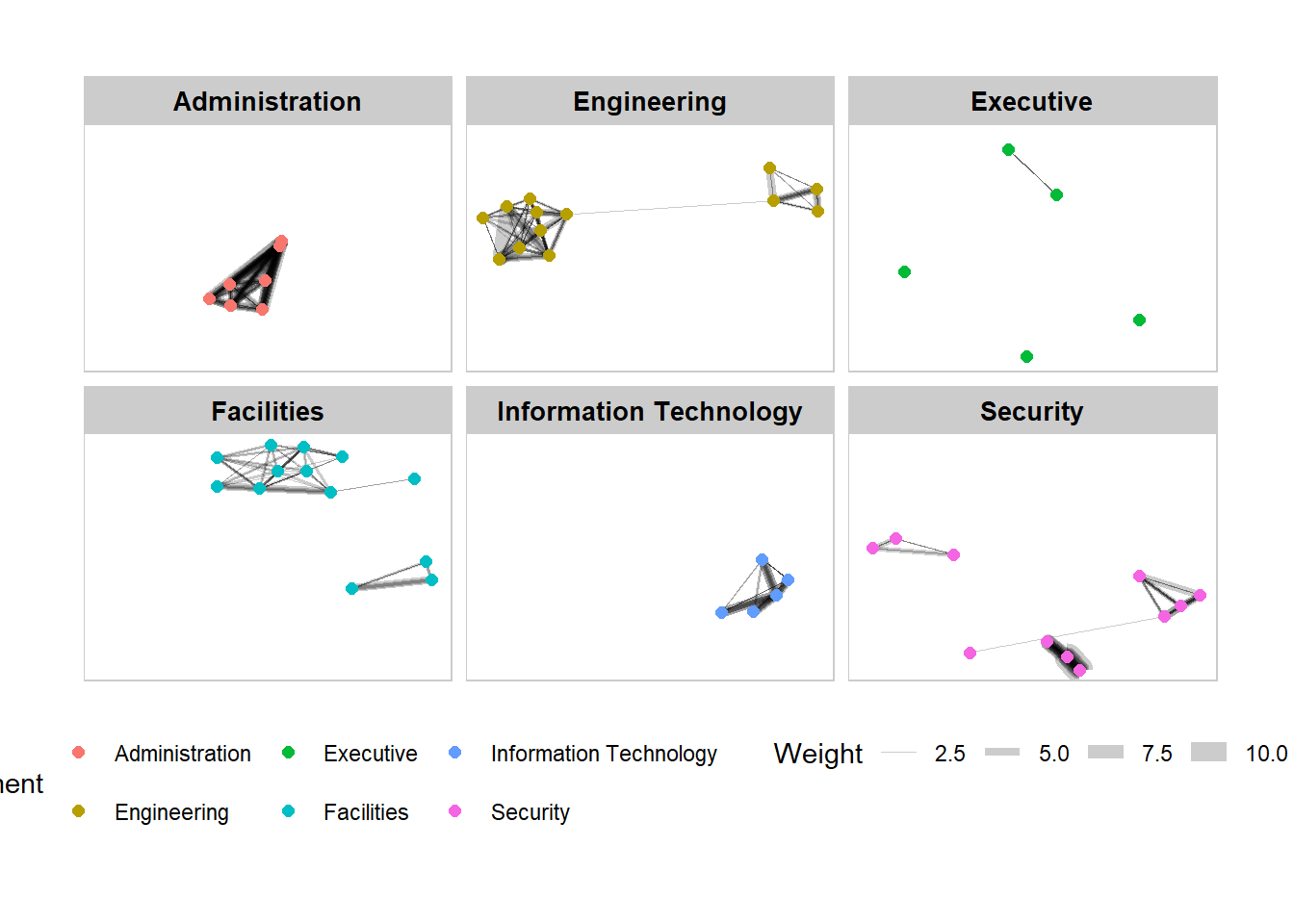
Network Metrics Analysis
Computing centrality indices
g <- GAStech_graph %>%
  mutate(betweenness_centrality = centrality_betweenness()) %>%
  ggraph(layout = "fr") +
  geom_edge_link(aes(width=Weight),
                 alpha=0.2) +
  scale_edge_width(range = c(0.1, 5)) +
  geom_node_point(aes(colour = Department,
            size=betweenness_centrality))
g + theme_graph()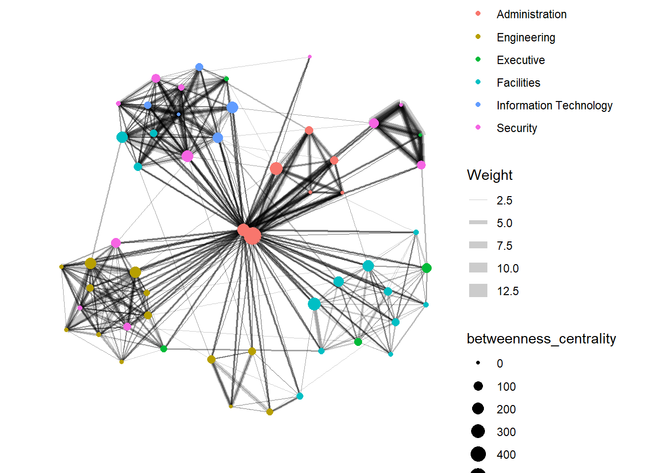
Visualising network metrics
g <- GAStech_graph %>%
  ggraph(layout = "fr") +
  geom_edge_link(aes(width=Weight),
                 alpha=0.2) +
  scale_edge_width(range = c(0.1, 5)) +
  geom_node_point(aes(colour = Department,
                      size = centrality_betweenness()))
g + theme_graph()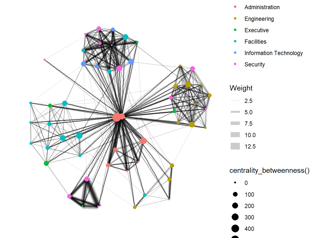
Visualising Community
g <- GAStech_graph %>%
  mutate(community = as.factor(
    group_edge_betweenness(
      weights = Weight,
      directed = TRUE))) %>%
  ggraph(layout = "fr") +
  geom_edge_link(
    aes(
      width=Weight),
    alpha=0.2) +
  scale_edge_width(
    range = c(0.1, 5)) +
  geom_node_point(
    aes(colour = community))

g + theme_graph()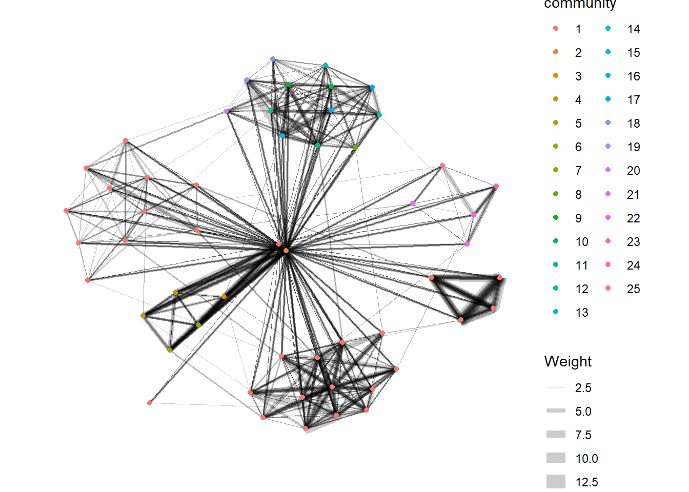
g <- GAStech_graph %>%
  activate(nodes) %>%
  mutate(community = as.factor(
    group_optimal(weights = Weight)),
         betweenness_measure = centrality_betweenness()) %>%
  ggraph(layout = "fr") +
  geom_mark_hull(
    aes(x, y,
        group = community,
        fill = community),
    alpha = 0.2,
    expand = unit(0.3, "cm"),  # Expand
    radius = unit(0.3, "cm")  # Smoothness
  ) +
  geom_edge_link(aes(width=Weight),
                 alpha=0.2) +
  scale_edge_width(range = c(0.1, 5)) +
  geom_node_point(aes(fill = Department,
                      size = betweenness_measure),
                      color = "black",
                      shape = 21)

g + theme_graph()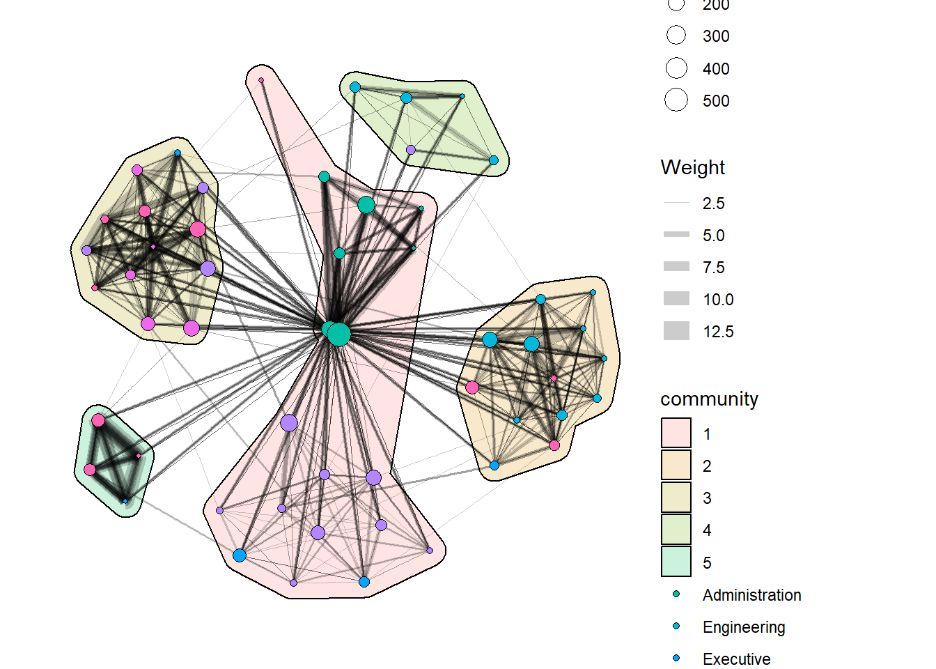
Building Interactive Network Graph with visNetwork
Data preparation
GAStech_edges_aggregated <- GAStech_edges %>%
  left_join(GAStech_nodes, by = c("sourceLabel" = "label")) %>%
  rename(from = id) %>%
  left_join(GAStech_nodes, by = c("targetLabel" = "label")) %>%
  rename(to = id) %>%
  filter(MainSubject == "Work related") %>%
  group_by(from, to) %>%
    summarise(weight = n()) %>%
  filter(from!=to) %>%
  filter(weight > 1) %>%
  ungroup()
Plotting the first interactive network graph
visNetwork(GAStech_nodes,
           GAStech_edges_aggregated)
Working with layout
visNetwork(GAStech_nodes,
           GAStech_edges_aggregated) %>%
  visIgraphLayout(layout = "layout_with_fr")
Working with visual attributes - Nodes
GAStech_nodes <- GAStech_nodes %>%
rename(group = Department) visNetwork(GAStech_nodes,
GAStech_edges_aggregated) %>%
visIgraphLayout(layout = "layout_with_fr") %>%
visLegend() %>%
visLayout(randomSeed = 123)Working with visual attributes - Edges
visNetwork(GAStech_nodes,
           GAStech_edges_aggregated) %>%
  visIgraphLayout(layout = "layout_with_fr") %>%
  visEdges(arrows = "to",
           smooth = list(enabled = TRUE,
                         type = "curvedCW")) %>%
  visLegend() %>%
  visLayout(randomSeed = 123)
Interactivity
visNetwork(GAStech_nodes,
           GAStech_edges_aggregated) %>%
  visIgraphLayout(layout = "layout_with_fr") %>%
  visOptions(highlightNearest = TRUE,
             nodesIdSelection = TRUE) %>%
  visLegend() %>%
  visLayout(randomSeed = 123)